Bar Charts and Histograms
The text below is a transcript of the video above, edited with AI assistance for clarity and flow. Where the two differ, the video is the authoritative version.
At 7:02, the video says that the mean roughly divides the area of the bars into the part above it and the part below it. That is the property of the median.
You’ll learn to
You have been learning how to summarise a distribution by knowing what the mean, the median, the standard deviation and the variance are and, for frequency tables of nominal variables, by knowing what the mode, the most frequent category, is. Now you are going to learn how to visualise that information. When we look at a graph, we often gather more information in a shorter amount of time than when we look at the summary statistics. Knowing both is important to get a sense of how a variable is distributed. In this video you will learn to:
- Choose and interpret bar charts and histograms for univariate data.
General Election vote: Frequency table
Let’s start with the British Election Study, which asked: which party did you vote for in the general election?
| 2024 General Election vote | Freq. | Percent | Cum. |
|---|---|---|---|
| Labour | 895 | 43.74 | 43.74 |
| Conservatives | 408 | 19.94 | 63.69 |
| Liberal Democrats | 224 | 10.95 | 74.63 |
| Scottish National Party (SNP) | 75 | 3.67 | 78.30 |
| Plaid Cymru | 22 | 1.08 | 79.37 |
| Green Party | 148 | 7.23 | 86.61 |
| Reform UK | 221 | 10.80 | 97.41 |
| Other (WRITE IN) | 20 | 0.98 | 98.39 |
| An independent candidate | 33 | 1.61 | 100.00 |
| Total | 2,046 | 100.00 |
This is the frequency table. It gives the numbers of people who said that they voted for each of those parties.
General Election vote: Frequency bar chart
The frequency table can be visualised with a bar chart.
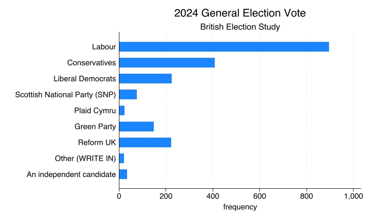
Here you have the frequency on the horizontal axis, and the vertical axis has the parties. The frequency denotes the number of observations: the number of people who responded that they voted for each of those political parties. You can see clearly that more than 800 people said that they voted Labour in the 2024 general election. Out of all of those who were interviewed, 895 did, so almost 900. That is why the Labour bar ends between the 800 and the 1,000 marks on the horizontal axis.
Frequency bar charts
A frequency bar chart is useful for visualising the distributions of nominal variables. The party that someone voted for in an election is a nominal variable. The chart shows how many observations are in each category: in this case, how many people said they voted for each party.
The order of the bars here does not make a difference, and it is important to keep that in mind. If we were to shuffle the order in which those parties appear and put, say, the Green Party or Reform UK at the top, that would not substantially change what the chart is communicating. This is something that distinguishes the frequency bar chart from the histogram, which comes next.
NSS Data: Summary
Before showing the histogram, let’s think back to the National Student Survey (NSS) satisfaction data, specifically question 28: “Overall, I am satisfied with the quality of the course”. The rate measures the share of students who responded either agree or strongly agree.
| Q28 | |
|---|---|
| Obs | 1,051 |
| Mean | 82.3 |
| Std. dev. | 12 |
| Min | 11.8 |
| Max | 100 |
There are 1,051 courses in the dataset. When you take the satisfaction rates of all of them, sum them up and divide by the number of observations, 1,051, you get a mean of 82.3. The standard deviation is approximately 12. As for the minimum, the course with the lowest approval rate has only 11.8% of students saying that they were satisfied with the quality of the course. And there are a few courses where every single student is satisfied: 100% satisfaction rates.
This is a summary table. It sums up the distribution in numbers: the number of observations, the mean, the standard deviation, the minimum and the maximum.
NSS Data: Histogram
This is the plot that allows us to visualise and illustrate this distribution.
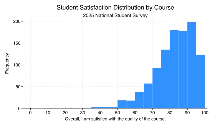
Notice how the horizontal axis, the x-axis, has different ranges of approval rates. They increase by five, so each bar has a width of 5 percentage points.
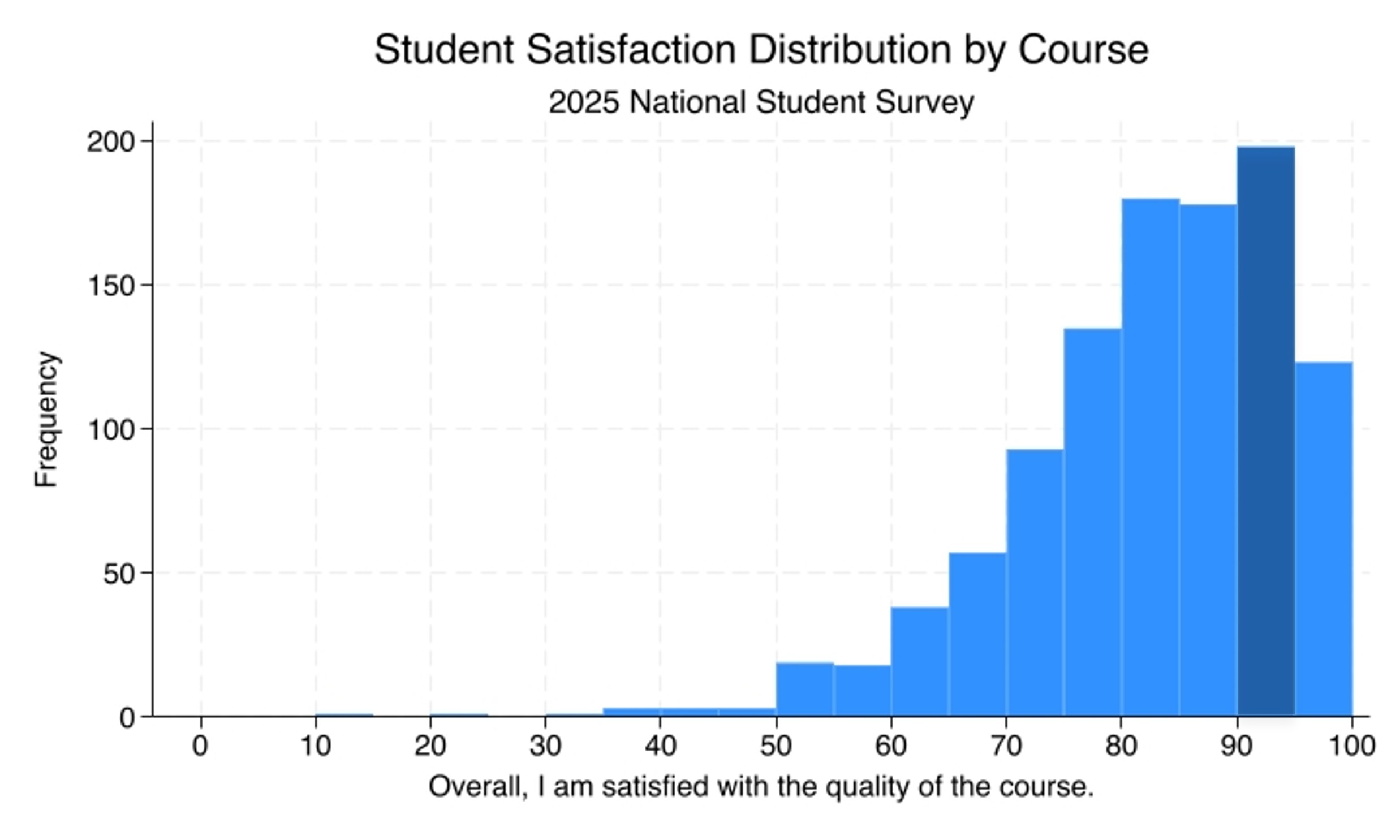
The shaded bar contains the number of courses with approval rates between 90% and 95%. If you look at the vertical axis, the frequency, the bar reaches up to 200. So there are about 200 courses between 90% and 95% satisfaction rates. The histogram allows us to visualise the entire distribution of approval rates across the 1,051 courses that the NSS has data for.
Histograms
Histograms are good for visualising distributions of ordinal, interval, and ratio variables. They show how many observations are in each range of values.
Here the order of the bars does make a difference. We could not just shuffle around the bars that are displayed along the horizontal axis, because that would completely change how we interpret the data. The order of the bars really means something here.
When you look at the mean and then at the histogram, it makes sense that the mean would be in the bar that comes right after 80.
Another variable: GDP per capita
Let’s look at another variable, so that you can map different distributions to different histograms. Here you have GDP per capita by country.
| Country | GDP per capita |
|---|---|
| USA | $58.4k |
| UK | $38.4k |
| China | $19.2k |
| Brazil | $14.6k |
| India | $7.7k |
| Ethiopia | $2.3k |
This is a snapshot of six countries, to illustrate that GDP per capita has a distribution that is more spread out: its standard deviation is larger relative to the mean than in the distribution of approval rates. There are big discrepancies between the GDP per capita of countries.
GDP per capita: summary
| GDPpc | |
|---|---|
| Obs | 162 |
| Mean | 19,619 |
| Std. dev. | 20,986 |
| Min | 596 |
| Max | 149,171 |
Notice here that the standard deviation is even larger than the mean. Remember that for the approval rates by course we have a mean of 82 and a standard deviation of 12. In this distribution, where there is more discrepancy between the values, the standard deviation is even bigger than the mean.
GDP per capita: Histogram
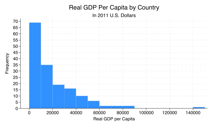
When you look at the histogram you can really tell, because some countries have a GDP per capita that is far above the mean. The mean here is about 19,000, and there are those few countries that are way above it.
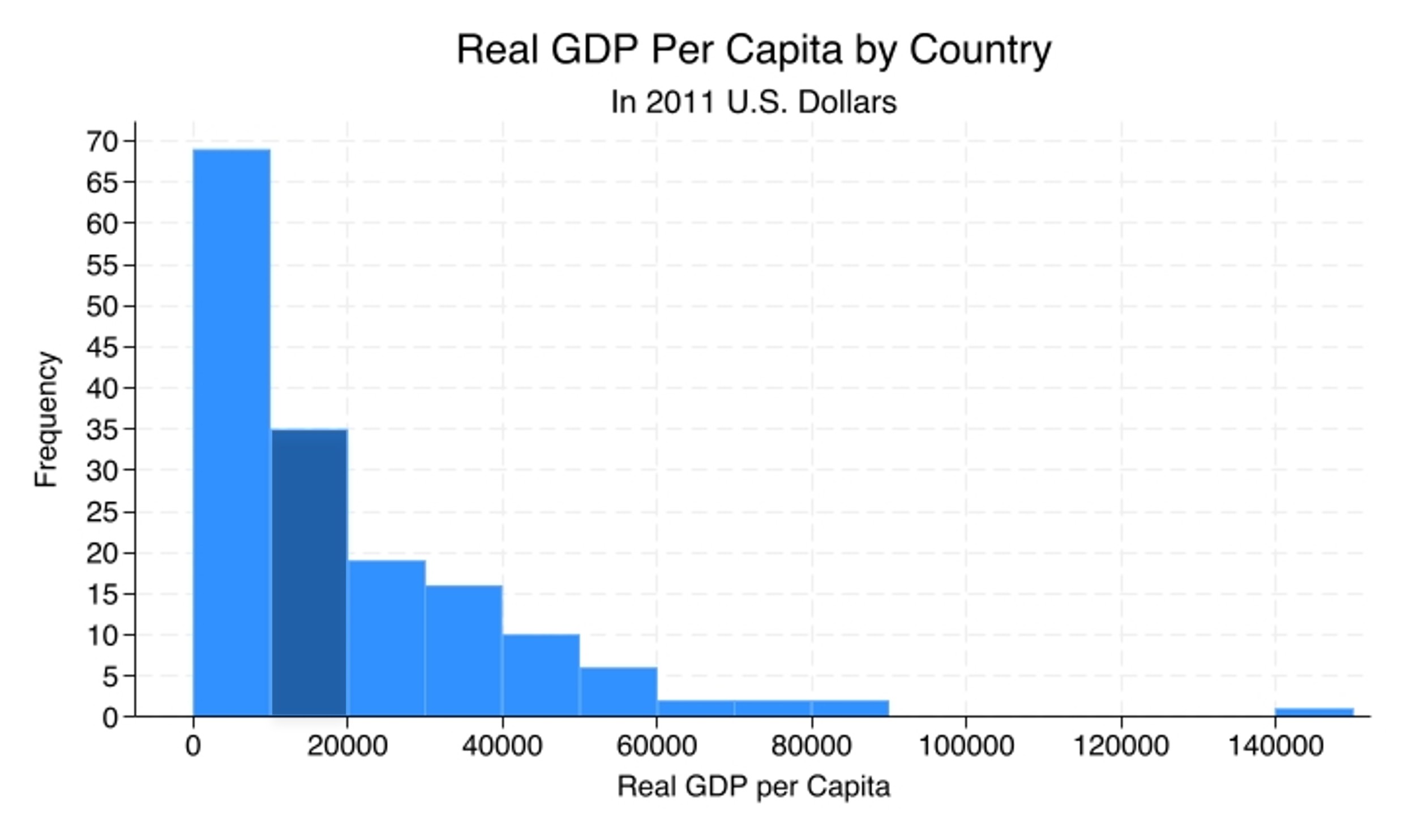
The histogram is telling you that there are 35 countries between $10k and $20k of GDP per capita per year.
Recap
- Bar charts and histograms visualise distributions.
- Bar charts are used for nominal variables and show counts by category.
- Histograms are used for ordinal, interval, and ratio variables and show counts within ranges of values.
Why this matters
The wrong type of graph, for example a histogram for a nominal variable, produces a data visualisation that is just plain wrong: one that obscures patterns or suggests structure that is not really there. The right visualisation helps us understand what is typical, what is rare, how spread out the distribution is, and how large the discrepancies between the values are. It complements the numbers that we get from summary statistics tables and frequency tables, so that we better understand the data we are going to analyse.