Describing Correlations in Stata
The text below is a transcript of the video above, edited with AI assistance for clarity and flow. Where the two differ, the video is the authoritative version.
You’ll learn to
Now that you know how to choose the appropriate plots and tables to analyse correlations between variables, it is time to learn how to do that in Stata. You will learn to:
- Generate and interpret bivariate summaries in Stata.
Materials
We use the British Election Study, which is available in the Shared Project Folder.
- The dataset is
British_Election_Study_2024.dta, in thedata-rawfolder. If you have not already, download it and save it into thedata-rawfolder on your own computer. - The do-file with the commands used here is
bivariate-bes.do, in thedofolder. Save it into your owndofolder.
When you download something, by default it goes to your downloads folder. For the commands to work, you need to have each file in the right folder: the dataset in data-raw and the do-file in do.
Insert the path to your folder on your computer
Remember that the do-files we provide contain a line that sets the working directory to the Shared Project Folder on my computer. That “address” only works on my computer. You need to replace it with the command that sets the working directory on your computer, so that the rest of bivariate-bes.do can work.
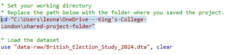
A reminder about how to do that. In Stata, click File, then Change working directory, and choose the folder you are using for your own analysis. I click on my shared project folder and click OK. What then shows up is cd followed by the path to this folder on my computer, in quotation marks. I can right-click this line in the command history and copy it. When I paste it into the do-file, it is exactly the same as the line already there, because this is my computer. When you do that on your computer, it is going to be different, and that is the line you use to replace the one in the do-file.
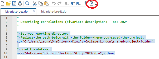
Select the top portion of the do-file and click “execute (do)”
After the working directory line is changed, you can select the top portion of the do-file and click execute. That opens the dataset.
Check if it has worked and save your do-file
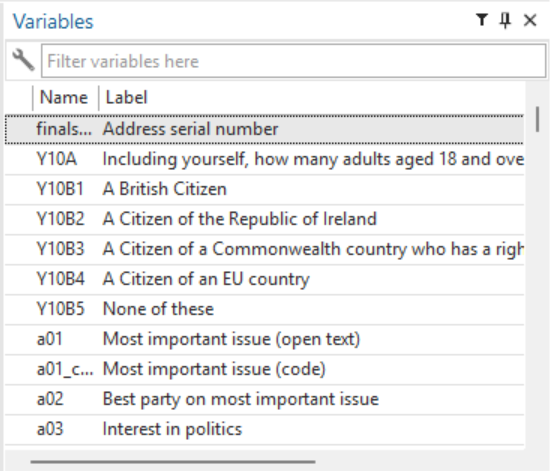
You will then see the variables listed, and if you click on Browse you see the dataset for the British Election Study. If you see that box on the top right with the list of variables, it means it has worked. Be sure to save your do-file in your do folder.
Read through the do-file comments and execute the commands
You can then read through the do-file comments and execute the commands. This do-file is your companion for learning how to describe bivariate relationships in Stata. Together with bivariate-brexit.do, it covers three types of bivariate analysis, depending on the variable types involved.
What is bivariate analysis?
Bivariate analysis is when you are analysing two variables and whether they go together. Univariate analysis is when we analyse the distribution of one variable at a time. Bivariate analysis, by contrast, describes the relationship between two variables.
The right tool for bivariate analysis depends on the types of variables being analysed. In the do-file you see several examples of cases, with the types of plots and tables appropriate for each combination of variable types.
Case 1: Nominal + Nominal
When you have two nominal variables, in our example gender and vote choice, the right tools are the cross-tabulation and the grouped (bivariate) bar chart. You use tabulate with the column option for percentages, and a bar chart command with the asyvars option for the grouped bar chart. The video uses catplot for the chart; the do-files use graph hbar instead. The output is equivalent.
In the do-file editor you see that I start with univariate descriptions, looking at one variable only. First is the univariate description of vote choice: the table and the plot with the number of people who said they voted for each party in the British Election Study.
Notice that when you start to work with a do-file you have three windows: the do-file itself, the window where the charts appear, and the main Stata window, where the tables and results appear and where you have the list of variables.
The next portion of the do-file gives you the gender distribution: the plot, and the table with the frequencies and percentages. There are a few more univariate distributions further down, for ideology and favourite newspaper, which we will see later.
I go straight to the chunk labelled as correlations between nominal variables: gender and vote choice. These are the commands that produce the cross-tabulation and the grouped bar chart.
tabulate b02 y09, column

graph hbar (count), over(y09) over(b02) asyvars
Whenever you have two nominal variables, you can use that as a template for your analysis.
Case 2: Nominal + Numeric
In the second case we have one nominal variable and one numeric variable: here, newspaper readership and ideology. This is where we compare means, using by with summarize to calculate the group means, and graph hbar with over() to visualise the differences: the mean ideology by favourite newspaper.
Back in the do-file, further up, I first work on the histogram for ideology. A numeric variable requires a histogram. You can follow the do-file to understand what each line is doing; the green text contains comments. This is the distribution of self-placed ideology, with about a thousand people placing themselves at five on a scale from 0 to 10, where 0 means left and 10 means right. Then there is the distribution of favourite newspaper: the number of people who declared that their favourite newspaper is the Guardian, the Mail, the category “other”, and so on.
Further down is the chunk of the do-file that compares means. To see the mean ideology by newspaper, you sort and then use by:
sort k03
by k03: summarize e01
These are the names of the variables in the dataset: e01 is how ideology is named and k03 is how the favourite newspaper is named. That is something you can check in the codebook. In the output you can see, for example, that the mean for Times readers is 5.29 and for Telegraph readers it is 6.4, and you have that information for each newspaper.
The next line shows the bar chart of means without any polishing. The axis title simply says “mean of e01”.
graph hbar e01, over(k03)After that comes the command that generates a properly formatted graph. You can follow the additional parts, the title, the subtitle and so on, which are added to make the chart more presentable.
graph hbar e01, over(k03) title("Favourite Newspaper and Ideology") subtitle("British Election Study, 2024") ytitle("Mean self-placed ideology (0 = Left; 10 = Right)") name(bes_news_ideol, replace)Case 3: Numeric + Numeric
Now we have numeric and numeric: the import shock and the Brexit vote share. The tools are the scatterplot and the regression line. For this we use a different do-file, bivariate-brexit.do.
Once you select the top chunk and run it, having changed the working directory line of course, you see that there is a new dataset loaded. This time it is the Brexit dataset. The do-file starts with a series of histograms. I ask you to follow through the do-file and understand what each part is doing; the comments should help you with that.
Then comes the step-by-step for the scatterplot. Use twoway (scatter) to plot individual observations. When you run just this, you produce the scatterplot without the regression line:
twoway (scatter leave_share import_shock)Once you start to add things, as the comments narrate, you get the regression line by adding (lfit), and then you start polishing the scatterplot.
twoway (scatter leave_share import_shock) (lfit leave_share import_shock)So the do-file has a version without the regression line and a version with the regression line. These are some examples of how to make those charts in Stata.
Interpreting scatterplots and regression lines
The scatterplot shows individual data points, and the regression line summarises the overall pattern.
- Direction: if you see an upward slope, it is a positive association; a downward slope is a negative association.
- Strength: the closer the points are to the line, the stronger the relationship between the two variables.
Your turn: Explore bivariate relationships
This is something to try for yourself. Work through the first two cases in bivariate-bes.do and the third, with additional scatterplot examples, in bivariate-brexit.do. Use the do-files as a starting point, and then explore bivariate relationships between different variables, using their content as a template.
Recap
- Cross-tabulations and grouped bar charts describe associations between nominal variables.
- Bar charts of means summarise differences in a numeric variable across categories.
- Scatterplots and regression lines summarise relationships between two numeric variables.
Why this matters
Describing relationships between variables is the foundation for asking why those relationships exist. Choosing the wrong tool for the wrong variable types produces meaningless or misleading output: Stata will do it if you ask it to produce a type of plot that is not correct for the variables you are analysing. And these skills are going to be very important for interpreting the bivariate analyses you might encounter in research papers, reports, and public debate.