Regression Analysis: Introduction
The text below is a transcript of the video above, edited with AI assistance for clarity and flow. Where the two differ, the video is the authoritative version.
You’ll learn to
Regression analysis is one of the most important statistical methods that social scientists use to analyse data. In this video you will learn to:
- Recognise a regression equation as a linear function.
- Read a scatterplot with a regression line.
- Use a regression equation to generate predicted values.
Scatterplots and regression lines
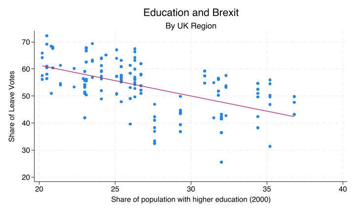
You are now familiar with this image: a scatterplot with a regression line drawn through it, the line of best fit. Scatterplots show the relationship between two numeric variables. The line is the regression line, and it comes from an equation. Now we start to learn what this equation looks like and how we can come up with predictions using it.
Linear functions: the general form
The regression equation is very similar to the linear function that you have encountered earlier in your education. Here we have a function where y is a function of x, in such a way that y is equal to a plus b times x:
\[y = a + bx\]
- a is the intercept: the value of y when x is zero.
- b is the slope: how much y changes for each one-unit increase in x.
A simple example
An example is the function that states that y is equal to 5 plus 2 times x:
\[y = 5 + 2x\]
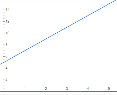
Here you have the linear equation and its graph, and from them we can determine the value of y for each value of x.
- If x = 0, y = 5 + 2(0) = 5. This is where the line cuts the vertical axis, the y-axis.
- If x = 1, y = 5 + 2(1) = 7.
- If x = 3, y = 5 + 2(3) = 11.
A regression has the same form as this simple example: each value of x gives us a predicted value of y.
A regression equation is a linear function
In a regression equation, we estimate the intercept and the slope that best fit the observations. The regression estimates the a and the b, which we then use to construct an equation where the value of one variable is used to predict the value of a different variable.
The result is a linear equation, with the same form as y = a + bx. But in a regression equation the y and the x are variables: y is the dependent variable and x is the independent variable.
The Brexit example
In the Brexit example, we can ask the question: do areas with more graduates vote differently on Brexit? That is, do areas with different percentages of people with higher education vote differently?
- y (dependent variable): the share of Leave votes. It goes on the vertical axis.
- x (independent variable): the share of the population with higher education, as a percentage of the population of each region of the UK.
Education and Brexit
This is the scatterplot that shows education and the Brexit vote.
Reading the plot
Each dot represents a UK region. The share of the population with higher education is on the x-axis and the share of Leave votes in the 2016 referendum is on the y-axis, so the two variables are cast along the two axes of the scatterplot.
The regression line runs through the cloud of dots. It is the line that best fits that cloud of dots; how we get to that line is something you will learn later. The line in this scatterplot runs downward, so there is a negative relationship: the higher the share of the population with higher education, the lower the share of Leave votes. You can see clearly, from the line that cuts through the cloud of dots, the negative correlation between the share of the population with higher education and the share of Leave votes in the Brexit referendum. This is the relationship that the regression equation captures.
The regression equation
This is the regression equation with the Leave share as y and the proportion of people with higher education as x:
\[\widehat{\text{Leave}} = 84 - 1.13 \times \text{HigherEd}\]
The intercept is approximately 84 and the slope is approximately −1.13. Notice the minus sign: as you increase the proportion of people with higher education, you decrease the predicted percentage of people who voted Leave in that region.
Generating predictions
We can then start plugging in numbers and get predictions.
- If HigherEd = 20%: 84 − 1.13(20) ≈ 61% Leave. For a region of the UK where 20% of people have higher education, you plug that into the equation and get a predicted Leave share of 61%.
- If HigherEd = 30%: 84 − 1.13(30) ≈ 50% Leave. You plug in 30% and get a predicted Leave vote share of 50%.
Predictions are approximations
These predictions are approximations. Not all regions where the higher education share is 20% have a Leave vote share of 61%. If you go back to the scatterplot and look at 20 on the x-axis, you will see a dot close to 20 that is right on the line, just as the regression line predicts, but you will also see a lot of dots that are somewhat distant from the line. With this one piece of information you can never get the exact share of Leave votes, but you can approximate it. Those predictions are the approximations that a regression allows us to make.
That is because education is not the only factor that shapes the Leave vote. There are other factors. The regression summarises the average tendency; it does not allow us to get the exact number for each dot.
Recap
- A regression equation is a linear function fitted to the data, fitted to the scatterplot.
- It has an intercept, the value of y when x is zero, and a slope, the change in y per unit of x.
- We use it to generate predicted values of y given any value of x.
Why this matters
Regression turns a visual pattern into a way to forecast the value of one variable depending on a different variable. It generates a precise, testable statement. Everything we look at from now on builds on this foundation of modelling one variable according to another. This is the very first step towards understanding regression analysis: from here you will learn more about different quantities, uncertainty, inference, and everything surrounding regression analysis.