Bar Charts and Histograms in Stata
The text below is a transcript of the video above, edited with AI assistance for clarity and flow. Where the two differ, the video is the authoritative version.
You’ll learn to
It is now time to start creating bar charts and histograms in Stata. In this video you will learn to:
- Create bar charts and histograms in Stata and use them to describe distributions.
Materials
We use the British Election Study, which is available in the Shared Project Folder.
- The dataset is
British_Election_Study_2024.dta, in thedata-rawfolder. If you have not already, save it into thedata-rawfolder on your own computer. - There is a new do-file. Alongside the one for summarising the British Election Study, the
dofolder hasvisualise-bes.do. Download it and save it into your owndofolder.
Insert the path to your folder on your computer
One line of visualise-bes.do has an “address” that only works on my computer. Replace it with the path to the project folder on your computer.
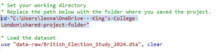
Select the top portion of the do-file and click “execute (do)”
Once you have replaced the path in the line that sets the working directory, you can run the top portion of the do-file. That will load the dataset.
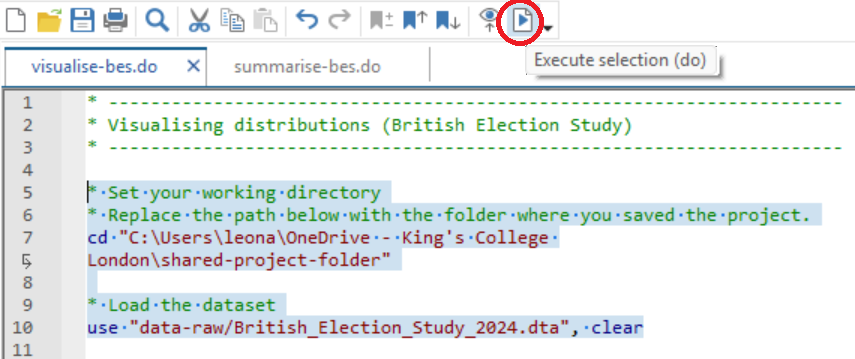
Check if it has worked and save your do-file
If you see the list of variables on the top-right pane of your Stata screen, it has worked. Be sure to save your do-file in your do folder.
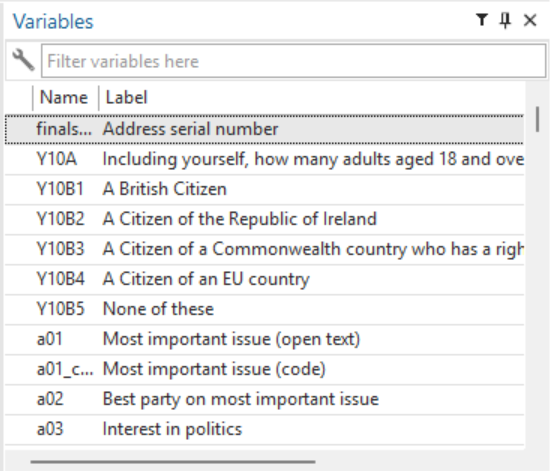
Read through the do-file comments and execute the commands
Now we can move on to creating histograms and frequency bar charts. The green text in the do-file is comments, and if you follow those comments carefully you will see that I am building a histogram step by step.
The finished histogram
You do not need to include every step along the way in order to get the histogram we are going to generate. To show you this, I select just the last histogram command:
hist Age if Age >= 0, width(5) start(15) xlabel(20(10)100) frequency title("Distribution of respondents' ages") subtitle("2024 British Election Study") name(age_hist, replace)This shows the distribution of respondents’ ages in the 2024 British Election Study. You can see, for example, that about 200 respondents are aged between 50 and 55. This is the clean and formatted version of the histogram. For pedagogical purposes, though, the do-file goes step by step, adding the different pieces of instruction until we get to the nicely formatted histogram.
Building it step by step
If you just run hist Age, you get the bare-bones version.
hist AgeIt did not drop the −2s. A −2 means that the respondent refused to answer, and we did not tell Stata to ignore those values, so they are in there. It is also difficult to make sense of the data in this version. The width of the bins is not clear: we cannot really tell how many years are included in each bar, or what range of values it covers. And the bars are not well aligned with the tick labels on the horizontal axis.
So first we drop the −2s. The result is still not that easy to read.
hist Age if Age >= 0Next we set the bin width to five.
hist Age if Age >= 0, width(5)Then we make sure that the histogram starts at 15, so that the bins align with the tick labels.
hist Age if Age >= 0, width(5) start(15)In the next line we change the information on the axis to make it more useful, with more labels and more signposting on the x-axis.
hist Age if Age >= 0, width(5) start(15) xlabel(20(10)100)Finally, frequency makes the histogram report not the proportion of respondents but the number of respondents.
hist Age if Age >= 0, width(5) start(15) xlabel(20(10)100) frequencyNow we can see that 200 respondents in the British Election Study are between 50 and 55 years of age. I encourage you to do this by yourself and read the comments.
The bar chart
For the bar chart, I went straight to creating the full chart of the general election vote.
graph hbar (count), over(b02) title("2024 General Election Vote") subtitle("British Election Study") name(bes_vote_bar, replace)The do-file also explains how to save the image into your output folder.
graph export "output/bes_vote_bar.jpg", as(jpg) name(bes_vote_bar) quality(100) replaceYour turn: Find additional variables to visualise
histgives us histograms.graph hbar (count), over()gives us the frequency bar charts.
Save the do-file on your computer and go through it, looking at the graphs it produces. Then I recommend that you explore the British Election Study data and codebook to look for additional variables to visualise.
Got tired of the BES? There’s more!
There are additional do-files and additional datasets in the Shared Project Folder that you can also explore if you are keen. This is the histogram of real GDP per capita by country.
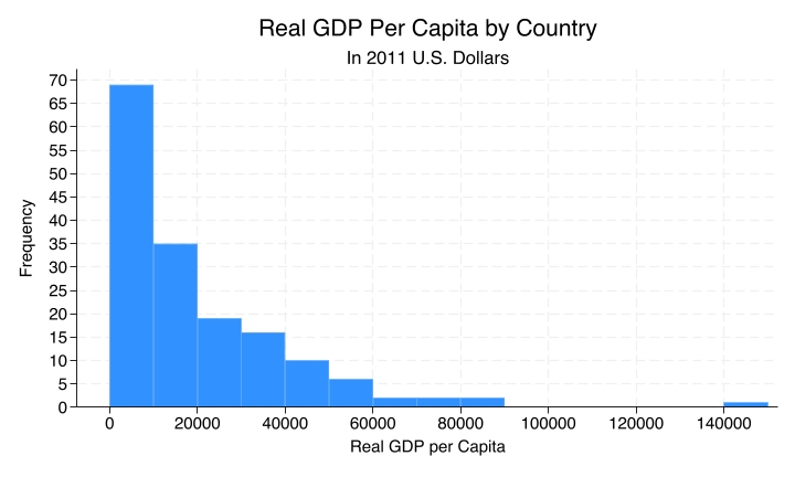
histogram-gdp.do has the code for this histogram. It uses the Quality of Government dataset, so be sure to download Quality_of_Government_2026.dta first. The codebook is there as well.
Still bored? There’s even more!
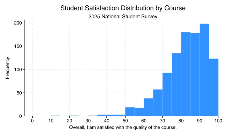
Similarly for the National Student Survey: the code that produces this histogram of student satisfaction by course is in histogram-nss.do. Be sure to download National_Student_Survey_2025.dta first. The codebook is also available.
Fancy a challenge?
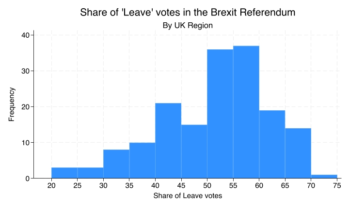
Finally, if you want a challenge, you can try to reproduce this histogram, which I made using the Brexit dataset. The dataset is there and the codebook is there, so you can come up with your own do-file and try to generate this exact histogram to test what you have learned about histograms in Stata.
Recap
- Frequency bar charts are used for nominal variables and show counts by category.
- Histograms, by contrast, are used for ordinal, interval, and ratio variables and show counts within ranges of values.
Why this matters
Graphs help us see patterns that are hard to spot in tables alone, and choosing the wrong type of graph can hide important features or suggest structure that is not there.
So remember: we want histograms for certain types of variables and frequency bar charts for other types. If you tell Stata to produce the wrong plot for the type of variable, it will do it for you, and you will end up with a figure that does not make a lot of sense. It is one of the duties of the analyst to be aware of those differences and to be able to map the different types of variables onto the different types of charts.