Summarising Distributions in Stata
The text below is a transcript of the video above, edited with AI assistance for clarity and flow. Where the two differ, the video is the authoritative version.
You’ll learn to
Now that you have learned about summary statistics tables and frequency tables, it is time to produce them in Stata. In this video you will learn to:
- Produce summary statistics and frequency tables in Stata and interpret what they show.
Materials
We use the British Election Study, which is available in the Shared Project Folder.
- The dataset is
British_Election_Study_2024.dta, in thedata-rawfolder. The codebook is in the same folder. I recommend downloading both and saving them into thedata-rawfolder on your own computer. - The do-file with the commands used here is
summarise-bes.do, in thedofolder. Save it into your owndofolder.
Remember that the idea is for you to replicate the folder structure of the Shared Project Folder on your own computer: each file you download goes into the folder with the same name in your local copy. Once the do-file is saved in your do folder, double-click it and Stata opens with the do-file ready.
Insert the path to your folder on your computer
The next step is to replace one line of the do-file you have downloaded. The line that sets the working directory has an “address” that only works on my computer. Replace it with the path to the folder where you saved your project: the “address” of the project folder on your computer.
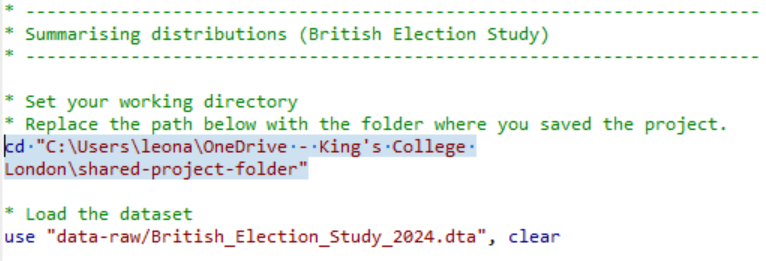
Select the top portion of the do-file and click “execute (do)”
There is one thing to know about do-files: if you select just a portion of the code and then click “execute selection (do)”, Stata will only execute that part. Here, selecting and running the top portion loads the British Election Study dataset.
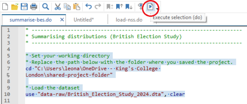
Check if it has worked and save your do-file
If you see the list of variables on the top-right pane of your Stata screen, it has worked. After you have replaced the path with the one to the project folder on your computer and run the top portion of the do-file, be sure to save your do-file in your do folder.
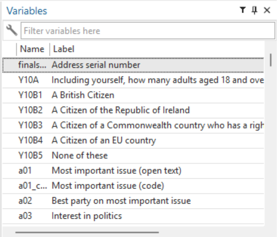
Read through the do-file comments and execute the commands
What you do now is follow through the do-file. It is your companion for learning how to produce summary statistics and frequency tables. Now that the top part has worked on your computer, we get to the real data analysis part.
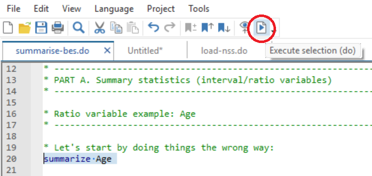
Summary statistics: age
summarize AgeIf you run summarize Age, you get a summary statistics table with the number of observations, the mean and the standard deviation. However, something is off: the minimum is −2. Why? Does it mean that people who were not even born were answering the British Election Study? No. This is where the importance of the codebook becomes visible.
Open the PDF with the British Election Study codebook and search for “age”, using Ctrl+F on Windows or Command+F on a Mac. You will find the part of the codebook with the question “Can you please tell me your age at your last birthday?”. It turns out that some people refused to reveal their age, and that was coded as −2. So if you just run summarize Age, some people are counted with an age of −2, and the mean is underestimated because of that. −2 is not really the age of these people; it is there because they refused.
Because we know the codebook, we know how to fix this: summarise age only if age is greater than or equal to zero.
summarize Age if Age >= 0Once we do that, the minimum age is 18 and the mean is 52 instead of 51. The smaller number of observations means that we have excluded the 60 people in the sample who refused to reveal their age.
Summary statistics: ideology
For ideology there is a similar coding scheme, where negative numbers mean that people refused to answer. In the codebook the variable is e01: the 0 to 10 self-placement on the left-right ideology scale.
summarize e01 if e01 >= 0Here you have 2,677 responses, a mean of 4.75, a standard deviation of 1.95, a minimum of 0 and a maximum of 10.
These are the summary statistics tables. Age is the example of a ratio variable, and ideology is the example of an interval variable.
Frequency tables
Then you have frequency tables. The first is for the education level, where you get both the number of people with each level of qualification and the percentages.
tabulate edlevelSimilarly, you can have a table like that for the general election vote: the party that respondents voted for.
tabulate b02Your turn: Find additional variables to summarise
You have seen that summarize gives us the mean and standard deviation, along with the number of observations, the minimum and the maximum (summary statistics), and that tabulate gives us frequency tables.
What I propose is that you explore the British Election Study data and codebook to look for additional variables to summarise. Open the codebook PDF and you will see that there are plenty of variables to explore. For example, there is a variable for whether the respondent is married, living with a partner, and so on. But notice that there you would probably have to instruct Stata to ignore the −999, because that value means that they did not state their status.
Recap
- In this video, you learned how to summarise distributions in Stata.
- Interpreting output requires checking for non-substantive values, such as the −2s for age, and understanding what each statistic represents.
- Be sure to choose the right type of table for the type of variable: nominal and ordinal variables, and interval and ratio variables, each have their appropriate summaries.
Why this matters
Summary statistics and frequency tables help you understand what is typical, what is rare, and whether values make sense. They allow us to detect problems in the data before moving on to graphs or statistical models. This type of initial data exploration is going to be very important.