Regression Slope
The text below is a transcript of the video above, edited with AI assistance for clarity and flow. Where the two differ, the video is the authoritative version.
The video calls the residual “the error” or “the error term”. The error term is a different thing: the distance from the true line, which we never observe, not from the estimated one.
You’ll learn to
Understanding where the regression slope comes from gives you an intuition for how to read a regression equation. In this video you will learn to:
- Identify the intercept and the slope in a regression equation.
- Explain where the slope comes from.
- Interpret the slope and the intercept in substantive terms.
Where we left off
We start from a regression equation that predicts the Leave vote share in the Brexit referendum. The idea is that you can approximate the Leave vote share in any given region of the UK by knowing the share of people in that region who hold a higher education qualification.
\[\widehat{\text{Leave}} = 84 - 1.13 \times \text{HigherEd}\]
The hat means predicted. The equation tells you that the predicted Leave vote share is 84 minus 1.13 times the share of people in the region with higher education. It is a linear function fitted to the data. The question then becomes: where do these numbers come from? How do we calculate the 84 and the −1.13?
The components of a regression equation
A regression has this general form:
\[\hat{y} = \hat{\beta}_0 + \hat{\beta}_1 x\]
- \(\hat{y}\) is the predicted value of the dependent variable.
- \(x\) is the independent variable, in this case the share of the population with higher education.
- \(\hat{\beta}_0\) is the intercept.
- \(\hat{\beta}_1\) is the slope.
The hats on the betas mean estimated. There is a difference between the estimated value and the real one, which comes up later; for now, read the hat as “estimated”.
You will also see the intercept called the constant. The two terms are used interchangeably: in the context of a regression, intercept and constant refer to the same thing, the \(\hat{\beta}_0\) in the equation. Likewise, you will see the term coefficient used as a substitute for slope. Here we call them intercept and slope, but know that the intercept can be called the constant and the slope can be called a coefficient.
Where does the slope come from?
The slope is calculated by dividing the covariance of x and y by the variance of x:
\[\hat{\beta}_1 = \frac{\text{Cov}(X, Y)}{\text{Var}(X)}\]
The covariance of x and y captures whether, and to what extent, the two variables move together. If they move together strongly in a positive way, you get a large positive number. If they move together strongly in a negative way, you get a large negative number. If they do not move together at all, you get a number close to zero.
The denominator is the variance of x, which you should already be familiar with: it is how spread out x is. So you take how x and y vary together, divide by how spread out x is, and you arrive at the estimated slope, \(\hat{\beta}_1\).
Intuition behind the formula
If x and y tend to move in the same direction, the slope is positive. If they tend to move in opposite directions, the slope is negative. We then scale by the variance of x so that the slope is expressed in the right units.
Interpreting the slope
For every one-unit increase in x, the change we expect to see in y is the estimated slope, \(\hat{\beta}_1\).
The sign of the slope tells us whether we are looking at a positive or a negative association: whether an increase in one variable is associated with an increase or with a decrease in the other. The size of the slope, how far it is from zero, tells us how much y is expected to change for a one-unit change in x.
Slope: Brexit example
\[\hat{\beta}_1 = -1.13\]
In the Brexit example the slope is −1.13. For each 1 percentage point increase in the higher education share, the Leave share is expected to decrease by 1.13 percentage points.
One thing to note: we are talking about percentage points on both sides, but that is not because regressions always describe relationships between percentage points. It is simply a feature of this example, where both variables happen to be measured in percentage points. One is the percentage of people with higher education degrees and the other is the percentage of votes for Leave. The percentage-point wording is not built into regression.
Where does the intercept come from?
This is the equation that gives us the intercept:
\[\hat{\beta}_0 = \bar{y} - \hat{\beta}_1 \bar{x}\]
Here \(\bar{y}\) is the mean of the dependent variable and \(\bar{x}\) is the mean of the independent variable. Once we know the slope, we multiply it by the mean of the independent variable, and subtract that result from the mean of the dependent variable.
Interpreting the intercept
The intercept is the predicted value of y when x is zero. Often that is not a meaningful real-world scenario, because in a lot of cases x being zero simply does not happen. The role of the intercept is to anchor the line. It is not something to over-interpret when reading a regression equation.
Intercept: Brexit example
\[\hat{\beta}_0 = 84\]
Read literally, the intercept says that if there were a region of the UK with a 0% higher education share, about 84% of people in that region would have voted Leave. But no region of the UK has a higher education share of zero. As the scatterplot below shows, the minimum is around 20%. A value of zero is entirely outside the data, so the intercept is a mathematical anchor, not a substantive prediction.
Residuals: the line is never perfect
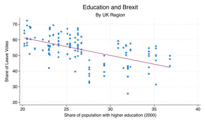
Another thing to keep in mind is the residuals. The line is never perfect. Only a handful of dots appear to lie exactly on the regression line. For just about every other region there is a distance between the dot and the line. That vertical distance is the residual: it is the error in the prediction.
For every region there is a difference between the actual Leave vote and the predicted value. Even the dots that look as if they sit exactly on the line most likely have a very small error; an error of exactly zero is very rare. You will never have a situation where every dot is exactly on the line. There are always residuals in a regression.
Larger residuals mean the regression predicts that region less well. The regions furthest from the line are the ones the regression does a poor job of predicting. For example, among regions with a higher education share between 30% and 35%, there is one where the regression equation would have predicted a much higher share of Leave votes than actually occurred: it sits far below the line, under 30% Leave. So for some regions the Leave share is well predicted by the share of the population with higher education, and for others it is poorly predicted.
Ordinary Least Squares
The slope and the intercept are calculated in a way that minimises the sum of squared residuals. This is a built-in property of the formulas: they make the sum of the squares of those residuals as small as possible.
This quantity is called the Residual Sum of Squares (RSS). It is an important concept for understanding what a regression does. And because the intercept and slope minimise that quantity, the most standard form of regression is called Ordinary Least Squares, or OLS. You will see regressions referred to as OLS in publications and reports, and this is the reason for the name.
Recap
- The slope is the covariance of x and y divided by the variance of x. It is how y changes per unit of x.
- The intercept is the predicted y when x is zero.
- OLS, Ordinary Least Squares, finds the line that minimises the sum of squared residuals, where the residuals are the vertical distances between each dot and the regression line.
Why this matters
Every regression result you read in a paper or a report rests on these calculations. Knowing what the slope captures helps you evaluate whether a result makes sense. And OLS is the standard estimation method across the social sciences.