Bivariate Regression in Stata
The text below is a transcript of the video above, edited with AI assistance for clarity and flow. Where the two differ, the video is the authoritative version.
You’ll learn to
It is now time to learn how to run and interpret a regression in Stata. You will learn to:
- Run a bivariate regression in Stata.
- Read the output: the slope, the intercept, the p-value, the 95% confidence interval around the slope, and the R-squared.
- Assess whether a regression result is statistically significant.
Materials
We use the Brexit Regional dataset, which is available in the Shared Project Folder.
- The dataset is
Brexit_Regional.dta, in thedata-rawfolder. Save it into thedata-rawfolder on your own computer. - The do-file with the commands used here is
regression-brexit.do, in thedofolder. Save it into your owndofolder.
Load the dataset
As always, the first commands set the working directory to your project folder and load the dataset.
cd "C:\Users\leona\OneDrive - King's College London\methods-education\shared-project-folder"

use "data-raw/Brexit_Regional.dta", clear
Replace the path in cd with the location of the project folder on your own computer. Once the commands run, the dataset is loaded with all of its variables.
You can follow along in the do-file, executing the commands as the video moves through them. We run two regressions: one that is statistically significant and one that is not.
From inference to regression
Before regression, we worked with differences in means and differences in proportions. We tested whether two groups differ in a mean or in a proportion: we measured the difference across groups, constructed a confidence interval around it, and obtained a p-value under the null hypothesis that the difference is zero. We then used the confidence interval and the p-value to test that hypothesis.
Now we describe and test a linear relationship between two numeric variables. The logic carries over: we test whether the real slope is zero, even when the estimated slope we find is not zero.
Regression 1: Education and the Leave vote
The running example is the relationship between education and the share of Leave votes across regions of the UK.
- Research question: Do regions where a higher proportion of the population has higher education vote Leave less?
- H0: There is no linear relationship between the higher education share and the Leave vote share.
- H1: As the proportion of people with higher education increases, the Leave vote share decreases.
Step 1: Produce the scatterplot
This is the simpler version of the command that generates the scatterplot with a fitted line:
twoway (scatter leave_share share_high_skill) ///
       (lfit leave_share share_high_skill), leg(off)
If you compare it with the do-file, you will see that the do-file version has more after leg(off): a y-axis title, a title, a subtitle, and a name for the graph, which sets it up to be saved by the command on the next line.
twoway (scatter leave_share share_high_skill) (lfit leave_share share_high_skill), leg(off) ytitle("Share of Leave Votes") title("Education and Brexit") subtitle("By UK Region") name(brexit_educ_scatter_line, replace)

graph export "output/brexit_educ_scatter_line.jpg", as(jpg) name(brexit_educ_scatter_line) quality(100) replace
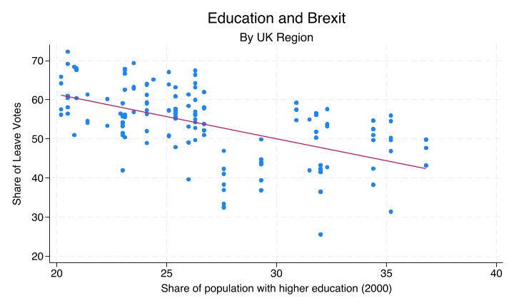
Running these produces and saves the scatterplot, “Education and Brexit, by UK region”. Each dot is a UK region and the line shows the estimated linear relationship. It is always a good idea to look at a scatterplot alongside a regression.
Step 2: Run the regression
The command that runs the regression is quite straightforward. You type regress, which can also be abbreviated to reg, then the dependent variable, then the independent variable. That is it.
regress leave_share share_high_skillHere leave_share is the dependent variable (y) and share_high_skill is the independent variable (x).
Reading the output: the coefficient table
| Element | What it tells you |
|---|---|
Coefficient |
Estimated slope (β̂₁) or intercept (β̂₀) |
P>|t| |
p-value |
[95% conf. interval] |
Plausible range for the true coefficient |
The Coefficient column gives you the estimated slope and the estimated intercept. The slope is on the row labelled with the independent variable, share_high_skill. The intercept is on the row Stata prints as _cons, because the intercept is also called the constant.
The p-value and the 95% confidence interval for the slope are printed on the same row. The p-value is displayed as 0.000. That does not mean it is exactly zero. It means that any non-zero digits come after the third decimal place: it is a remarkably small p-value. The 95% confidence interval tells us that the range of plausible values for the slope runs from about −1.42 to about −0.84.
Reading the output: top-right block
| Element | What it tells you |
|---|---|
Number of obs |
Sample size used in the regression |
R-squared |
Share of variance in y explained by x |
In the top-right block of the output you find the number of observations, which here is the number of regions included in the regression, and the R-squared, which is around 0.30.
Writing the regression equation
This is how you carry those quantities from the Stata output into an equation.
_cons≈ 83.92 is the intercept (β̂₀). Elsewhere this is rounded to 84; here we can be a bit more precise.share_high_skill≈ −1.13 is the slope (β̂₁).
\[\widehat{\text{Leave}} = 83.92 - 1.13 \times \text{HigherEd}\]
The hat means predicted. You take the intercept, and add the slope multiplied by the percentage of people in the region with higher education. The result is the predicted Leave vote share.
Interpreting the slope
For each 1 percentage point increase in the higher education share, the Leave share is expected to decrease by 1.13 percentage points. The negative sign indicates that the greater the share of people with higher education in a region, the lower the share of Leave votes in the Brexit referendum, which matches the direction seen in the scatterplot.
Assessing statistical significance
- The p-value is well below the 0.05 threshold.
- The 95% confidence interval, [−1.42, −0.84], lies entirely below zero. It does not include zero, so zero is not a plausible value for the real slope.
We therefore reject the null hypothesis and conclude that the relationship is statistically significant.
Reporting R-squared
The R-squared tells us that about 30% of the variance in the Leave share is explained by the education share. The remaining 70% is explained by other factors that are not included in this model.
Regression 2: Unemployment and the Leave vote
Now a different regression. We could ask: do regions with higher unemployment vote Leave more? One hypothesis is that yes, in regions with higher unemployment people felt more disaffected, more like protesting against the status quo, and more motivated to vote Leave. The null hypothesis is that there is no relationship between unemployment and the Leave vote: a zero slope, a flat line.
The procedure is the same, with one change to the command. Instead of regressing leave_share on share_high_skill, you regress it on unemployment. It is good practice to generate the scatterplot and regression line first:
twoway (scatter leave_share unemployment) (lfit leave_share unemployment), leg(off) ytitle("Share of Leave Votes") title("Unemployment and Brexit") subtitle("By UK Region") name(brexit_unemp_scatter_line, replace)The plot already suggests that the result is not going to be statistically significant. The line is very flat. It is very slightly positive, but it looks as though the 95% confidence interval will include zero. And it does.
reg leave_share unemploymentThe do-file uses reg here, the abbreviated version of regress. It works just the same.
Reading the output: non-significant result
| Element | Value | Interpretation |
|---|---|---|
| Slope | +0.19 | Small positive estimate |
| p-value | 0.655 | Much larger than 0.05 |
| 95% CI | [−0.64, +1.02] | Includes zero |
| R-squared | 0.001 | Near-zero explanatory power |
The coefficient for unemployment is about 0.19. However, the p-value is 0.655. The probability of observing a result at least as extreme as this one, assuming that the null hypothesis is true, is 65.5%. That is quite a high probability, and it is consistent with a 95% confidence interval that includes zero: the lower limit is −0.64 and the upper limit is about 1, so zero is a plausible value for the slope.
The R-squared is very small: a tiny share of the variation in the Leave share is explained by unemployment. The output also tells you that there are 166 observations in this regression.
The decision rule: same logic, different outcome
The decision rule is the same; the outcome is different.
- The 95% confidence interval includes zero.
- The p-value is far above 0.05.
- The R-squared indicates near-zero explanatory power.
This is a non-significant result. We fail to reject the null hypothesis that there is no relationship between unemployment rates and the Leave vote share. The slope of 0.19 is consistent with chance variation in the data, rather than reflecting a true relationship.
Note. A simplification. Failing to reject the null hypothesis does not show that there is no relationship. It means only that these data do not give us enough evidence of one.
Recap
regress y x, with the dependent variable first and the independent variable second, fits a bivariate regression and produces the slope, the intercept, the p-value, the confidence interval, and the R-squared.- If the 95% confidence interval for the slope excludes zero, we reject the null hypothesis. Otherwise, we fail to reject it.
- The R-squared measures how much of the variation in the dependent variable is explained by the independent variable.
Why this matters
Regression is the core tool of quantitative social science. You will keep encountering regression tables in papers as you move along in your education, and knowing how to read and interpret them is a core skill in the social sciences.